Example for HV Calculation:
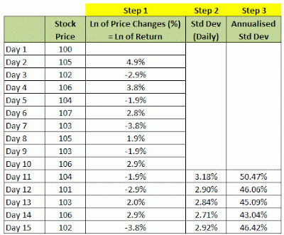
Suppose we have the daily stock price data and would want to calculate HV for 10-day period (10-day HV).
The daily stock price data is in the first two column of the table below:
Note:
Step 1, 2 and 3 in the table will be described below.
Steps to calculate Historical Volatility (using MS Excel):
Step 1: Calculate the Price Returns.
In this case for the above example, we use formula (4) mentioned in the earlier part (Part 2).
However, when the price change is quite small, the price returns calculated using formula (3) or (4) is quite similar.
Step 2: Calculate the Standard Deviation of the Price Returns, which will result in �Daily� Standard Deviation.
In MS Excel, formula �=STDDEV� can be used to calculate Standard Deviation as in formula (1) mentioned in Part 2.
If the period used for calculation is 10 days (like in the example), we�ll use the formula �=STDDEV� for a �rolling 10 days�.
Hence, the Standard Deviation for Day 11 will use Price Return data from Day 2 to Day 11; for Day 12 will be from Day 3 to Day 12; for Day 13 will be from Day 4 to Day 13, and so on.
Step 3: Annualise the �Daily� Standard Deviation in order to obtain the HV.
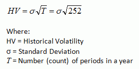
Since standard deviation is in daily and assuming there are 252 trading days in a year, we can annualise the �Daily� Standard Deviation by using the following formula:
Note:
Different number of days in a year may be used by different site, such as 254 days or 256 days.
252 days is the number of days used in ivolatility.com.
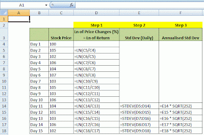
Here is the screen capture of the MS Excel formula used for the calculation in the table above.
Since HV is actually a standard deviation, in order to be able to interpret and use HV data better, it is good if we could have a better understanding on the concept of standard deviation, which will be discussed in the next part.
Continue to: Part 4: Understanding Standard Deviation
To view the list of all the series on �Historical Volatility�, please refer to:
Suppose we have the daily stock price data and would want to calculate HV for 10-day period (10-day HV).
The daily stock price data is in the first two column of the table below:

Note:
Step 1, 2 and 3 in the table will be described below.
Steps to calculate Historical Volatility (using MS Excel):
Step 1: Calculate the Price Returns.
In this case for the above example, we use formula (4) mentioned in the earlier part (Part 2).
However, when the price change is quite small, the price returns calculated using formula (3) or (4) is quite similar.
Step 2: Calculate the Standard Deviation of the Price Returns, which will result in �Daily� Standard Deviation.
In MS Excel, formula �=STDDEV� can be used to calculate Standard Deviation as in formula (1) mentioned in Part 2.
If the period used for calculation is 10 days (like in the example), we�ll use the formula �=STDDEV� for a �rolling 10 days�.
Hence, the Standard Deviation for Day 11 will use Price Return data from Day 2 to Day 11; for Day 12 will be from Day 3 to Day 12; for Day 13 will be from Day 4 to Day 13, and so on.
Step 3: Annualise the �Daily� Standard Deviation in order to obtain the HV.
Since standard deviation is in daily and assuming there are 252 trading days in a year, we can annualise the �Daily� Standard Deviation by using the following formula:

Note:
Different number of days in a year may be used by different site, such as 254 days or 256 days.
252 days is the number of days used in ivolatility.com.
Here is the screen capture of the MS Excel formula used for the calculation in the table above.

Since HV is actually a standard deviation, in order to be able to interpret and use HV data better, it is good if we could have a better understanding on the concept of standard deviation, which will be discussed in the next part.
Continue to: Part 4: Understanding Standard Deviation
To view the list of all the series on �Historical Volatility�, please refer to:
 2:01 AM
 killnine


